Climate Modelling IV: GCMs Study Case

In parts I to III of previous climate modelling posts, we commented general aspects of climate models, how they work and also the main challenges and difficulties facing modellers.  In this fourth and final part of this series of posts, I want to show you an interesting application of Global Circulation Models (GCMs).

In Asia, the Mekong River (see Figure below), which is the 12th longest river in the world with a length of 4,350 kilometres, represents a fundamental source of resources for different economic activities in Southeast Asia, such as agriculture and fishing. Another fundamental aspect to consider is the strong intervention of the river with large hydraulic projects, such as dams for hydropower generation. Due to the river represents a fundamental source of resources for the different cities and human settlements located in the basin, interesting studies have been carried out in order to assess the potential effects of climate change in the Mekong River.

Mekong River 

Kingstonet al. (2011) explored the potential effects of global environmental change on water resources in the Mekong river basin and they also proposed a method to estimate the uncertainty of this prediction. For this purpose, they integrated GCMs with hydrological modelling. This method represents a really interesting approach to predict potential effect of climate change on the environment; different disciplines working together in order to create more sophisticated tools.

In addition, another significant contribution was to consider different climate scenarios given by a GCMs structure. Basically, they built different GCM scenarios working as a base for a hydrological model (SLURP) of the study area. The fundamental strength of this methodology was to observe modelled responses of the freshwater behaviour due to different climate scenarios. Specifically, they generated different global warming scenarios between 0.5 and 6.0°C. For the 2°C scenario, they used seven different GCMs. Although there were clear similarities among the GCMs, it was useful to use different models structures to analyse the influence of these structures in the final projection uncertainty.

Mekong River 

According to the main purpose of the study, the effort of researchers was mainly focused on the understanding and measurement of the model uncertainty. An interesting result was to find a significant effect on the uncertainty due to the differences in precipitation projections given by the different GCMs, even for the same scenario. As we could see in the previous post, one of the most relevant challenges facing GCMs modellers is to improve precipitation and water cycle simulation. This was also emphasized by other researchers in a study developed with multiple GCMSs in India, where were found severe uncertainties in future rainfall estimations. Conversely, a proper consistency was found in GCMs projection for both snowmelt season and evapotranspiration in the Mekong river basin.

Finally, the most significant outcome was related to the strong dependence of hydrological behaviour in the basin (discharge) with potential changes in precipitation patterns. Due to the seven GCMs applied and considering the different precipitation estimations of these, for the 2°C scenario the parameters of the hydrological model were numerically estimated with an uncertainty between -2.0 – 2.0% and the discharge pattern was suitably represented by the model (see Figures below).

As we can see, the obtained results ratify the proposed methodology of applying different GCMs in order to obtain a suitable estimation of the final uncertainty, minimizing this value and finally obtaining better projections. 

Mekong River, Parameter Uncertainty for HadCM3 (GCM) Model, 2°C Scenario

Mekong River, Monthly Discharge for Base – Line and Seven GCMs Applied, 2°C Scenario

COP 21: Never Reach ......... 1,5°C

Today is a historic day for humanity!.

That is the headline of many newspapers and web pages which have been following the international conference on climate change (COP21) in Paris. Today it was presented the final draft which summarizes two week of negotiations by representatives from 195 countries.

One of the most significant agreements is about the new target for global warming temperature. As we noticed in the previous post, the target of 2°C meant the starting point of the discussion for this version of the conference. Due to scientific evidence given along COP21 sessions, this goal changed: it's essential to pursue a lower value, with special efforts to restrict the increment to 1,5°C. According to categorical simulations this new target represents a significant and favourable change of scenery regarding to the potential effect on the global environment.

Another interesting point is related to finance. The funding of $100 billion per year by developed countries to support environmental policies in developing countries will start operating by 2020. This represents a substantial measurement to promote an integral solution with developing and developed countries working together. A global threat necessarily requires being tackled with a common view.

Although this represent an important advance facing the global warming, it´s necessary to be aware about what 1,5°C means; this figure must be analysed again, and again. Seems to be clear that the effect on climate change should be significantly less and probably some extreme consequences may be avoided by 2100, however, it´s still a 1,5°C increment; which are the environmental effects of this new scenery?. As can we see, environmental models and their continued progress have undoubtedly been (and they will remain being) a major player.

I invite you to take a look to the COP21 web page and read in detail this already called “historic document”. 

 “If it is adopted, this text will mark a historic turning point” (Laurent Fabius, president of COP21)

COP 21: Never Reach 2°C

As many of you may already know, these days from November 30 to December 11 it is holding the international conference on climate change COP21 (21st Conference of Parties) in Paris. Authorities from United Nations are carrying out negotiations in order to define effective measurements to keep the level of global warming bellow 2°C by 2100. But, why this number?, why 2°C?.

Although the debate around this figure is quite complex, the video below offers an interactive explanation for this value defined in 2009 by the International Panel on Climate Change (IPCC) in Copenhagen. The video summarize relevant environmental phenomena identified in the last two centuries such as relationship between sea level and pH, CO2 and global temperature, dynamic of Arctic sea ice, greenhouse anthropogenic emissions and trade-related CO2 transfers.

For the special purpose of this blog, considering the different perspectives that we have been discussing here, it is absolutely interesting to visualize the essential role of environmental models underpinning the analysis and projections of potential temperature and precipitation anomalies by 2100 (and their massive consequences) for each studied scenario. 

Climate Modelling III: Global Climate Models (GCMs), Challenges of Modelling the Whole Planet

In the previous post we reviewed general concepts of climate modelling. In this post the GCMs approach will be analysed, which are mainly characterized by considering the largest possible scale in the environmental science: the entire Earth. As we already analysed in this blog, the discrete control volume or box is the minimum spatial unit to represent numerically the atmosphere over a specific portion of the land. In addition to other sources of error, the size of the box is directly related to the model accuracy (Wainwright and Mulligan, 2013).

Although the uncertainty of GCMs has been measured and defined as substantial (Palmer,2014), the identification of sources of uncertainty along the modelling process represents clear opportunities to improving GMCs. In this context, it is fundamental a suitable understanding of the limitations and challenges facing GMCs modellers. This viewpoint was emphasized by Burroughs (2007) who identified different potential areas to improve GMCs and minimize the uncertainty:

• Clouds: this area involves clouds formation processes, their properties absorbing and reflecting sunlight and better understanding of precipitation dynamics (see Figure below). In addition, the anthropogenic emission of particles, such as sulphur dioxide by fossil fuel consumption, leads to a disturbance in the natural balance of sunlight absorption and reflection processes. Moreover, there is still no clarity about the precise effect of this pollution phenomena on cloudiness (increase or decrease clouds cover). Thus, the main challenge is related to the definition of more accurate parameters in models to represent clouds dynamics at suitable space and time scales (Burroughs, 2007).
• Tropical cyclones: it is necessary an adequate representation of tropical cyclones intensity and their effects in energy fluxes processes. According to Burroughs (2007) the resolution of GMCs is unable to represent suitably this local phenomenon highly relevant to predict global warming.
• Land-surface dynamics: it is necessary a better understanding of the effect of some land variables on climate processes. For instance, weather models with considerable higher resolution have shown that appropriate handling of soil moisture data can lead to more accurate rainfall predictions. Therefore, more accurate description of physical features of the land, such as run off, stored precipitation and its interaction with the atmosphere will lead to a better representation between these and their effect on climate forecast (Burroughs, 2007).
• Winds, waves and water cycle: the representation of water cycle and the interaction between oceans and the atmosphere represent probably the most relevant source of uncertainties in GCMs (Palmer2014). Furthermore, the energy exchange between sea and the atmosphere is also essential for climate dynamics. Therefore, including a more detailed representation of this processes as well as an accurate analysis of physical interaction between winds and waves could represent a substantial improvement for climate models (Burroughs,2007).
• Greenhouse gas emission: the representation of multiple emissions of greenhouse gases (e.g. Carbon Dioxide (CO2), Methane (CH4) and Fluorinated gases (F-gases)) represents a relevant source of uncertainty in climate models, due to the dynamics of human activities and behaviour of these pollutant in the atmosphere.

-        

Simplified Scheme of Absorption and Reflection of Sunlight (Tour of the Electromagnetic Spectrum, NASA, 2014)

As can we see, the challenges to minimize the uncertainty of this powerful modelling tool could be summarized in two main ideas. Firstly, it is necessary to improve the knowledge in some relevant climate processes and define suitable parameterizations of these in GCMs. This effort implies not only a better understanding of complex chemical and physical processes through monitoring data but also requires an improvement in how monitoring activities should carried out for higher resolution scales. Secondly, as Neelin (2011) argues, a factor that must not be disregarded is the spatial and time scale and its close relationship with computational requirement, which are not necessarily available with current technology (Burroughs, 2007 and Palmer, 2014). 

Finally, it is relevant to highlight that some local climate processes may generate large scale effects, such as convective clouds dynamics (Palmer, 2014) and turbulence (WMO, 2015) which are not able to be represented in a typical GCMs horizontal resolution (around 100 km). In this context, Regional Climate Models (RCMs) are playing a fundamental role to understand local phenomena which GCMs are not able to represent (see Figure below). Indeed, both approaches working together represent a current solution. This and other solutions must be urgently explored due to climate models play an overriding role in the understanding and prediction of global environmental change.  

High Resolution Simulation of Convective Clouds System (Palmer,2014)

Climate Modelling II: How Climate Models work?

Climate change is happening. Several studies applying forecasts models, with a certain level of uncertainty, suggest that global warming will continue increasing exponentially in the next decades if rigorous measures are not taken. Although climate has historically changed with significant intensity (Burroughs, 2007), the current climate phenomena and its clear relationship with anthropogenic activities is probably the main concern for humanity today; the climate change is a threat. In this context, whereas an intense social, economic and political debate is taking place, climate models appear as an essential and complex tool in order to measure and predict the climate change.

The complexity of climate models lies in trying to represent atmospheric processes occurring at planetary scale for long periods of time, such as decades, centuries or even more. This leads to the main challenge for climate modellers: developing computer models with the necessary accuracy to recreate the planet climate (Burroughs,2007).

Climate models are based on fluid dynamic and thermodynamics laws (Stute et al., 2001, Neelin, 2011 and Wainwright and Mulligan, 2013). Due to climate dynamics is governed by physics laws, these environmental processes can be expressed as a set of equations that normally have no general solution. However, numerical approximations can be carried out using computational fluid dynamics models. A common approximation to solve this numeric representation of the atmosphere is to divide the domain or study area into discrete control volumes or boxes (see Figure below). This method, known as finite volume method, allows to represent each box through a set of partial differential equations whose formulation and solution is related to the values in the surrounding control volumes (Neelin, 2011 and Wainwright and Mulligan, 2013). Due to this approach is based on small boxes representing together the whole area of study, the size of the control volumes is crucial for the model accuracy. In effect, the error of the representativeness of the equation solutions in a specific cell is related to the box size (Wainwright and Mulligan, 2013). 

Grid Section for a Typical Climate Model (Neelin, 2011)

As we can imagine at this point, the spatial scale plays a significant role in the development of climate models. Different variables, equations, assumptions and model’s definitions are considered according to the size of the area of interest which could be a specific region or the whole planet. According to this is possible to distinguish two main approaches: Global Climate Models or Global Circulation Models (GCMs) and Regional Climate Models (RCMs) (see Figure below). While the first ones simulate the climate system at planetary scale in order to understand and forecast global phenomena, the second ones work at regional scales in order to explain local climate processes being also useful for policymaking (World Meteorological Organization WMO, 2015).

In the next posts we will review different application and study cases of GCM and RCM highlighting their main features, some challenges associated to their development and the implication of the time scale.  

Grid Approach for GCMs and RCMs (WMO, 2015)

Climate Modelling I: An Interesting Introduction

In the next posts we will be submerged in different existing approaches of climate modelling, probably the spinal core of a endless number of models currently used to predict the effect of global environmental change on our planet. Therefore, as an introduction, I recommend you to see this interesting talk given by Dr. Gavin Schmidt, Director of the NASA Goddard Institute for Space Studies (GISS).

During the lecture, called "The Emergent Patterns of Climate Change", two of the most relevant challenges related to climate modelling have been highlighted: first, the coexistence of multiple complex variables and second, the scale of modelling, from local phenomena until global simulations. Enjoy!

We Must Continue Monitoring Our Planet…

Environmental monitoring is probably one of the most relevant activities in continuous development in environmental sciences. Collected data is widely used to understand natural phenomena and their complex relationship with anthropogenic activities. Furthermore, as we saw in the previous post, data acquisition is playing a crucial role in models developing not only for validation processes, but also as input data for parameters definitions.

One appropriate question of using models to estimate the effects of climate change on biodiversity is; how accurate is the estimation or prediction of these effects? Normally, more accurate input data should entail less uncertainty of models. Even though there are many factors affecting the accuracy of models outcomes, such as user expertise, it is particularly significant the effect of observational datasets in models performance. Good examples of this can be found in models applied on biodiversity.In addition to technical challenges of monitoring activities, a huge challenge of collecting biosphere data is the inherent difficulty to measure significant variables. In effect, as Medvigy and Moorcroft (2011) argue, some relevant parameters to biosphere models are difficulty to obtain directly, like carbon distribution. As a solution to this, monitoring data can be used to estimate indirectly variables which are difficult to obtain through direct measurements. This is a significant contribution of monitoring data to environmental modelling and it represents a useful method in order to minimize models uncertainties (Medvigy and Moorcroft, 2011).

Estimated shift of vegetation gradient over a 30 years period, Santa Rosa Mountains, Southern California, USA (Breshears et Al, 2008)

It has also been recognized the needs of improving models introducing more detailed observational data, in this case, related to plant´s distribution patterns. As Thuiller et al. (2007) suggest, the introduction of vegetation dynamic data in models conceptualization represents an opportunity of improvement for Dynamic Global Vegetation Models (DGVMs). Indeed, the same Author assert that plants migration and their distribution patterns are consider relevant sources of uncertainties in prediction models in the climate change context. Similarly, Breshears et al.,2008 argue that some variables such as migration rates and variability in ecosystem properties are highly sensitive to climate change. Therefore, these variables should be carefully considered in models input and parameters definition.It seems to be clear that including monitoring data, such as patterns of plants distribution according to a desired scale of analysis, should lead to a reduction of uncertainties in the prediction of biodiversity response due to global environmental change. However, this requires a previous systematisation of complex information whose availability in a proper space and time scales, it is not ensured for every area of interest. We have to consider this before.

Modelling Biodiversity; Simulating a Complex Environmental Dynamic

It has widely been recognized that climate change produces effects in vegetation distribution (McMahon et al., 2011), therefore, different approaches have arisen in order to understand, measure and predict the effect of environmental change on the biosphere.

Dynamic Global Vegetation Models (DGVMs) have extensively been used to study the biodiversity dynamic (e.g. Sato, 2009, Moncrieff et al., 2015, Kucharik et al., 2006, and Halofsky et al., 2013). This approach integrates diverse knowledge of vegetation dynamics, including physiology and biogeochemistry, for different climate scenarios in order to predict vegetation and ecosystem changes due to climate change. Although these models represent advanced tools to develop biodiversity simulations, it has been argued that they are not able to obtain suitable results at landscapes scales (Hickler et al., 2004, Halofsky et al., 2013). An interesting study carried out by Halofsky et al., 2013 combines DGVMs approach with State and Transition Models (STMs). Although the last ones simulate vegetation changes by disturbances at local or landscape scales, normally these do not consider the effects by climate dynamics. This study offered a novel modelling approach combining the strengths of two different models families, in order to predict vegetation changes by climate change at landscape scale. The model showed satisfactory results which were contrasted with monitoring data available to the study area.

Forest inventory plots and potential vegetation in Oregon, obtained from DGVM-STM model; modal vegetation class estimated for 1971-2000 (recent historical) and forecast for 2100 (Halofsky et al., 2013)

Another interesting study was conducted by Medvigy and Moorcroft (2011) in the Harvard Forest, northeaster USA, and Quebec. The researchers assessed the performance and accuracy of a specific biosphere model called Ecosystem Demography Version 2 (ED2) whose outcomes were contrasted against biodiversity data obtained through a continuous monitoring in the study area for 11 years (see Figure below). The developed approach consisted in the application of two different models parameterizations; one of them using conventional setting (from literature) and a second one using parameters estimated with the available data from monitoring. According to the study, the second model had a better response than the conventional one, and it was proposed as a powerful tool to predict and forecast different biodiversity variables of interest in that specific area. 

Forest inventory: Northeaster USA (green) - Quebec (blue) (Medvigy and Moorcroft, 2011)

This approach represents an effective tool since the monitoring data was used not only in the validation process but also in the prediction parameters definition. However the lack of data could be a relevant restriction for this approach in areas without available and suitable information.

Similarly to DGVMs and STM models, the presented ED2 approach based fundamental processes of its development on biosphere data. This highlights the fundamental role of environmental monitoring in biodiversity modelling. In the next post we will analyse the relevance of the biosphere monitoring and its close relationship with the accuracy of biodiversity models.  

Environmental Modelling: Useful Tool for a Huge Concern

Nowadays, global environmental change probably represents one of the most important concerns on our planet. Thus, there has been growing interest from different stakeholders to understand the past, current and future processes linked with this global issue. In this context, environmental modelling plays a relevant role, not only as a useful tool to comprehend complex environmental phenomena but also because their outcomes are being used in the decision making carried on by relevant actors.

In this blog we will be discussing different interesting approaches to environmental processes using models, hence, as an introduction it is appropriate to highlight first the relevance of outcomes assessment. Given that models are abstractions of reality, it is necessary to point out that quality of input dataset, uncertainty, hypotheses as well as any theoretical definition underpinning the model must be considered as part of the results interpretation. Although normally scientists running a particular model have considerable knowledge of the weaknesses and strengths of this, the outcomes assessment is not trivial. Indeed, as Matthewset al. (2010) argued, it can be defined phases or typical evaluations for environmental modelling and software (EMS) outcomes. These commonly are peer review, validation, reliability, usability, relevance, interpretability and utility. Each of these instances of evaluation entails its own challenges, such as intangibility of EMS outputs or different results interpretations. 

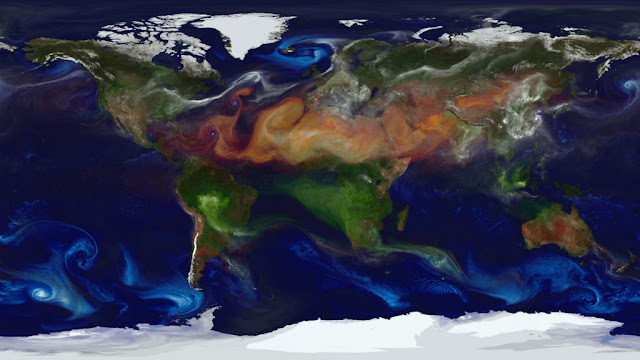
Figure 1. Colorful View of Aerosol Movement (Nasa, Goddard Space Flight Center, 2012) (video)

Models have become a useful and powerful tool for a huge concern, and their suitable application is also an enormous challenge. Therefore, I’m inviting anyone interested in any field within environmental science to enrich the discussion about modelling application and its role in the understanding of global environmental change.

‘Modelling is described as an art because it involves experience and intuition as well as the development of a set of mathematical skills’ (Wainwright and Mulligan, 2013).